Random Fourier Features

In the previous post, we introduced the idea of kernels as a way to lift a separation problem to a much larger space (potentially infinite-dimensional) while keeping the computation tractable via the “Kernel Trick.” We also mentioned that when the number of points in the dataset is very large—which is the case in most modern applications—the kernel method is less useful, as it requires computing and storing a huge $n \times n$ matrix.

The idea of the Random Fourier Features (RFF) method is that, in some cases, there is a very clean approximation of the kernel function that works on average for a random sample. Due to the concentration of measure phenomenon, the number of samples needed to ensure a very good approximation is surprisingly low. The idea was first proposed in a seminal paper by Rahimi and Recht [1].

Stationary Kernels

Note that our definitions of kernels can be generalized to include complex-valued kernels. This will matter for the theorem below, though for applications we ultimately care about the real-valued case.

We call a function $f:\mathbb{R}^{d}\to \mathbb{C}$ positive definite if the stationary kernel $K:\mathbb{R}^{d}\times \mathbb{R}^{d}\to \mathbb{C}$ defined by $K(x,y)=f(x-y)$ is positive definite. In the complex case, this means that for every choi}_ce of points $x_1 ,\ldots,x_n$ and scalars $c_1,\ldots,c_n$, it holds: $$\sum_{i=1}^n \sum_{j=1}^n c_i \cdot \overline{c_j}\cdot f(x_i-x_j)\ge 0$$

The Fourier Transform

The space of functions satisfying $\int_{\mathbb{R}^{d}}^{}{|\varphi(x)|}\ \mathrm{d}{x}<\infty$ is denoted by $L^1(\mathbb{R}^d)$. The Fourier transform of $f$ is always continuous and vanishes at infinity, meaning $\hat{f}(\xi)\to 0$ when $\| \xi \|\to \infty$. We denote the space of continuous and vanishing functions as $C_0(\mathbb{R}^d)$.

Recall that a continuous probability measure $\mu$ on $\mathbb{R}^{d}$ is defined by its probability density function $p:\mathbb{R}^{d}\to \mathbb{R}_{+}$. The expected value of a random variable $Z:\mathbb{R}^{d}\to \mathbb{C}$ with respect to $\mu$ is simply: $$\mathbb{E}[Z]=\int_{\mathbb{R}^{d}}^{}{Z(x)\cdot p(x)}\ \mathrm{d}{x}=\int_{\mathbb{R}^{d}}^{}{Z(x)}\ \mathrm{d}{\mu(x)}.$$ Therefore, integration against $\mu$ is the same as integrating with the standard Lebesgue measure weighted by the density function. The Fourier transform of $\mu$ is defined to be the Fourier transform of $p$: $$\widehat{\mu}(\xi)=\int_{\mathbb{R}^{d}}^{}{p(x)\cdot e^{-2\pi i\cdot \left\langle x,\xi \right\rangle}}\ \mathrm{d}{x}=\mathbb{E}_{x\sim \mu}[\exp(-2\pi i \left\langle x,\xi \right\rangle)].$$

This can be defined also for non-continuous probability measures, using the expectation notation. Without getting too much into measure theory, note that if $\mu$ is, say a discrete distribution, it has no probability density function. We can still write an integral against $\mu$, but this is the Lebesgue Integral, and not the classic Riemann integral over $\mathbb{R}^d$, and it might have a very different meaning (for example in the discrete case, it is a sum).

Bochner’s Theorem

We are now ready to state the main theorem connecting kernels to probability distributions:

Proof Sketch. ($\Rightarrow$) This direction is complicated, so I’ll only mention the key steps. A full proof can be found in [2].

1. Establish that the map $\widehat{g}\mapsto \int_{\mathbb{R}^{d}}^{}{g\cdot f}\ \mathrm{d}{x}$ is a continuous linear functional on the space $\mathcal{F}(L^{1}(\mathbb{R}^{d}))$, i.e., the image of absolutely integrable functions under the Fourier Transform.
2. Use the Gelfand-Naimark theorem, which says the Fourier transform of $L^{1}(\mathbb{R}^{d})$ is dense in $C_{0}(\mathbb{R}^{d})$ (continuous functions vanishing at infinity). By density, we extend our functional to a continuous linear functional $\Phi$ on all of $C_{0}(\mathbb{R}^{d})$.
3. Apply the Riesz-Markov Representation Theorem, which states that functionals on $C_{0}(\mathbb{R}^{d})$ correspond to measures. Thus, there exists a measure $\mu$ such that $\Phi(h)=\int_{\mathbb{R}^{d}}^{}{h}\ \mathrm{d}{\mu}$. This implies the integral representation of $f$, and further analysis shows $\mu$ is a probability measure.

($\Leftarrow$) This is the easier direction. Suppose $f(x)=\int_{\mathbb{R}^{d}}^{}{e^{-2\pi i \left\langle x,\xi \right\rangle}}\ \mathrm{d}{\mu(\xi)}$ for a probability measure $\mu$. Let $x_{1},\ldots,x_{n}\in\mathbb{R}^{d}$ and $c_{1},\ldots,c_{n}\in \mathbb{C}$. We check positive definiteness: $$\sum_{i,j=1}^{n}c_{i}\overline{c_{j}}f(x_{i}-x_{j})=\int_{\mathbb{R}^{d}}^{}{\sum_{i,j}c_{i}\overline{c_{j}} \cdot \exp(-2\pi i \left\langle x_{i}-x_{j},\xi \right\rangle)}\ \mathrm{d}{\mu(\xi)}.$$ Using exponent properties $\exp(-2\pi i \left\langle x_{i}-x_{j},\xi \right\rangle)=\exp(-2\pi i \left\langle x_{i},\xi \right\rangle)\cdot \overline{\exp(-2\pi i \left\langle x_{j},\xi \right\rangle)}$, we can rewrite the integral as: $$=\int_{\mathbb{R}^{d}}^{}{\left(\sum_{i}c_{i}e^{-2\pi i \left\langle x_{i},\xi \right\rangle}\right)\cdot \overline{\left(\sum_{j}c_{j}e^{-2\pi i \left\langle x_{j},\xi \right\rangle}\right)}}\ \mathrm{d}{\mu(\xi)}=\int_{\mathbb{R}^{d}}^{}{\left|\sum_{i}c_{i}e^{-2\pi i \left\langle x_{i},\xi \right\rangle}\right|^{2}}\ \mathrm{d}{\mu(\xi)}.$$ We have a non-negative integrand integrated against a non-negative measure, so the result is non-negative. Thus, $f$ is positive definite. $\blacksquare$

Random Fourier Features

Suppose we have a stationary kernel $K:\mathbb{R}^{d}\times \mathbb{R}^{d}\to \mathbb{R}$, defined by a function $f:\mathbb{R}^{d}\to \mathbb{R}$. Without loss of generality, assume $f(0)=1$ and $f$ is continuous. By Bochner’s Theorem, there is a probability measure $\mu$ such that $$f(\Delta)=\int_{\mathbb{R}^{d}}^{}{e^{-2\pi i \left\langle \Delta,\xi \right\rangle}}\ \mathrm{d}{\mu(\xi)}=\mathbb{E}_{\xi\sim \mu}[\exp(-2\pi i \left\langle \Delta,\xi \right\rangle)].$$ Writing $\Delta=x-y$, we have $$K(x,y)=f(x-y)=\mathbb{E}_{\xi}[\exp(-2\pi i \left\langle x-y,\xi \right\rangle)]=\mathbb{E}_{\xi}[e^{-2\pi i \left\langle x,\xi \right\rangle}\cdot \overline{e^{-2\pi i \left\langle y,\xi \right\rangle}}].$$ Thus, randomly drawing $\xi\sim \mu$ gives an estimator that equals $K(x,y)$ on average. However, there are two problems with this naive approach:

1. Variance: Drawing a single sample $\xi$ will have high variance.
2. Complex Numbers: The computation involves complex variables even though the kernel is real. We want a real-valued feature map.

Using Only Real Numbers

To deal with the second problem, we use the following trigonometric identity:

Proof. The product-to-sum formula gives $\cos(\varphi)\cos(\psi)=\frac{1}{2}[\cos(\varphi+\psi)+\cos(\varphi-\psi)]$. Applying this to $\varphi=\alpha+b$ and $\psi=\beta+b$: $$2\cos(\alpha+b)\cdot \cos(\beta+b)=\cos((\alpha+b)+(\beta+b))+\cos((\alpha+b)-(\beta+b)).$$ The second term is $\cos(\alpha-\beta)$, which is independent of $b$. The first term satisfies: $$\mathbb{E}_{b}[\cos(\alpha+\beta+2b)]=\frac{1}{2\pi}\int_{0}^{2\pi}{\cos(\alpha+\beta+2b)}\ \mathrm{d}{b}=\frac{1}{4\pi}\left[\sin(\alpha+\beta+2b)\right]_{0}^{2\pi}=0.$$ Therefore, $\mathbb{E}_{b}[\cos(\alpha+b)\cos (\beta+b)]=\frac{1}{2}\cos(\alpha-\beta)$. $\blacksquare$

Proof. Since $K$ is real-valued, we have $$K(x,y)=\Re(K(x,y))=\Re\left(\int_{\mathbb{R}^{d}}^{}{e^{-2\pi i \left\langle x-y,\xi \right\rangle}}\ \mathrm{d}{\mu(\xi)}\right)=\int_{\mathbb{R}^{d}}^{}{\cos(-2\pi \left\langle x-y,\xi \right\rangle)}\ \mathrm{d}{\mu(\xi)}.$$ By the previous lemma, setting $\alpha=-2\pi \left\langle x,\xi \right\rangle$ and $\beta=-2\pi \left\langle y,\xi \right\rangle$, we have $$\mathbb{E}_{b}[z(x)\cdot z(y)]=\mathbb{E}_{b}[2\cos(\alpha+b)\cos (\beta+b)]=\cos(\alpha-\beta)=\cos (-2\pi \left\langle x-y,\xi \right\rangle).$$ Taking the expectation over $\xi$, we obtain $\mathbb{E}_{\xi,b}[z(x)\cdot z(y)]=K(x,y)$. $\blacksquare$

Reducing the Variance

Recall that in randomized algorithms, Monte-Carlo algorithms run a fixed number of trials and return an answer that is correct with high probability. Concentration inequalities, like Hoeffding’s, Bernstein’s, and Chebyshev’s, formally answer the question: how likely is a random variable to attain a value far from its mean?

The special property of Hoeffding-type inequalities is that for sums of independent random variables, the concentration is exponentially strong. In other words, if a random variable $Y$ is the sum of a number of independent random variables $X_1,\ldots,X_n$, then $Y$ has very strong concentration properties.

This suggests the following Monte-Carlo estimate: $$E(x,y)=\frac{1}{R}\sum_{i=1}^{R}z_{i}(x)z_{i}(y),$$ where $z_{i}(x)=\sqrt{2}\cos(-2\pi \left\langle x, \xi_{i} \right\rangle +b_{i})$ with $\xi_{i}\sim \mu$ and $b_{i}\sim [0,2\pi]$ drawn independently. Let us formalize the quality of this estimator:

Proof. First, $\mathbb{E}[E(x,y)]=K(x,y)$ by linearity of expectation. Second, $E$ is the sum of $R$ i.i.d. random variables $X_{i}=\frac{1}{R}z_{i}(x)z_{i}(y)$. Note that $z_{i}(x)$ is bounded in $[-\sqrt{2},\sqrt{2}]$ because $\cos$ takes values in $[-1,1]$. Therefore, $|X_{i}|\le\frac{2}{R}$ almost surely, which implies the mean is also in this range. Hence $\left|X_{i}-\frac{K(x,y)}{R}\right|\le \frac{2}{R}$, and by Hoeffding’s inequality, $$\begin{aligned} \Pr(\left| E(x,y)-k(x,y) \right|)&=\Pr\left(\left|\sum_{i=1}^{R}X_{i}-R\cdot \frac{k(x,y)}{R}\right| \ge \varepsilon\right) \\ & \le 2\exp\left(-\frac{\varepsilon^{2}}{2R(2/R)^{2}}\right)=2\exp(-\varepsilon^{2}R/8). \end{aligned}$$ $\blacksquare$

This result can be upgraded to a uniform bound over a compact subset of $\mathbb{R}^{d}$. This means the samples $\xi_{1},\ldots,\xi_{R}$ and $b_{1},\ldots,b_{R}$ can be fixed once for the entire dataset and still approximate the kernel well for all pairs of points simultaneously.

Recap and Example

This procedure produces a random map: $$\mathbf{z}:\mathbb{R}^{d}\to \mathbb{R}^{R},\quad \mathbf{z}(x)=\frac{1}{\sqrt{R}}(z_{1}(x),\ldots,z_{R}(x)).$$ The features in $\mathbb{R}^{d}$ are replaced by random features in $\mathbb{R}^{R}$ that capture the same kernel interactions, meaning $$\left\langle \mathbf{z}(x),\mathbf{z}(y) \right\rangle\approx K(x,y).$$

Recall the example of the Radial Basis Function kernel from the previous post: $$K(x,y)=\exp\left(-\frac{1}{2\sigma^{2}}\left\lVert x-y \right\rVert^{2}\right).$$ This is a stationary kernel defined by the function $f(x)=\exp(-\frac{1}{2\sigma^{2}}\left\lVert x \right\rVert^{2})$. To determine the distribution $p(\xi)$ to sample from, we need to satisfy Bochner’s relation: $$f(x) = \int_{\mathbb{R}^d} p(\xi) e^{-2\pi i \langle x, \xi \rangle} d\xi = \hat{p}(x).$$ By the Fourier Inversion Theorem, $p$ must be the inverse Fourier transform of $f$. However, since the Gaussian function $f(x)$ is symmetric ($f(x)=f(-x)$), its inverse transform is identical to its forward transform. Thus, we can compute $p = \hat{f}$. The Fourier inversion can be applied because we are dealing with Gaussians, which are smooth and rapidly decaying functions (in the Schwartz space).

We need the following standard identity, asserting that the Fourier transform of a Gaussian is a Gaussian.

In our case, $f(x) = e^{-a|x|^2}$ where $a = \frac{1}{2\sigma^2}$. Plugging this into the Lemma: $$\begin{aligned} p(\xi) = \hat{f}(\xi) &= \left( \frac{\pi}{1/(2\sigma^2)} \right)^{d/2} \exp\left( -\frac{\pi^2 |\xi|^2}{1/(2\sigma^2)} \right) \ &= (2\pi \sigma^2)^{d/2} \exp\left( -2\pi^2 \sigma^2 |\xi|^2 \right). \end{aligned}$$

This looks like the probability density function of another Gaussian. Suppose it has variance $\tau^2$, then it satisfes $$\frac{1}{2\tau^2} = 2\pi^2 \sigma^2 \implies \tau = \frac{1}{2\pi \sigma}.$$

Thus, to approximate the Gaussian kernel with width $\sigma$, we must sample frequencies from: $$\xi \sim \mathcal{N}\left(0, \frac{1}{(2\pi \sigma)^2} I\right).$$

Let’s see this in action. In the next plot we have $10000$ points sampled from two circles. The linear model doesn’t work, and the full RBF kernel perfectly separates the data. However, the RBF kernel does computation based on the number of points, which is huge. Next we have Random Fourier features with $R=10,50,100,1000$ and we can see that even for $50$ the separation is almost perfect! This is a huge reduction in the runtime complexity. The diagrams show the decision boundaries of each classifier.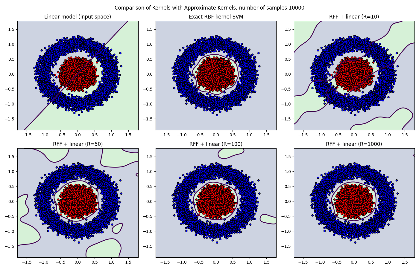

In the next post, we’ll discuss another randomized algorithm that approximates a specific family of kernels, called Polynomial kernels.

References

1. Rahimi, A., & Recht, B. (2007), Random Features for Large-Scale Kernel Machines .
2. Bell, J. (2015), Gaussian measures and Bochner’s theorem .