The Kernel Method

In this post, we will explore the idea of kernels in machine learning. In future posts, we will explore different ways to approximate specific kernel computations. Approximation is useful for big data applications due to the prohibitively high cost of exact kernel computations.

High Level Idea

Suppose we wish to find a linear separation rule $$f(x)=w^{\top }x$$ that minimizes some objective function. Since many datasets are not linearly separable (or even close to being so), a natural idea is to embed the dataset in a higher dimensional vector space in a specific way that ensures better separation. A classic example is separating circular data, as depicted below:

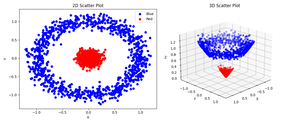
We map $\varphi:\mathbb{R}^{2}\to \mathbb{R}^{3}$ by setting $\varphi(x,y)=(x,y,\sqrt{x^{2}+y^{2}})$. Under this map, the datasets can be linearly separated by a plane.

Remark. For those unfamiliar with Hilbert spaces, these are just vector spaces with an inner product that are also complete (every Cauchy sequence converges). Finite-dimensional spaces are always Hilbert spaces, but we can also choose to work with infinite-dimensional spaces.

There are multiple problems we must solve for this approach to be useful:

1. Finding $h\in \mathcal{H}$ might be much harder than finding $w\in X$, since $\mathcal{H}$ might have a larger dimension (potentially infinite).
2. Computing $f(x)$ requires computing an inner product in $\mathcal{H}$, which is not necessarily efficient (or even computable).

Representer Theorem

To solve problem (1)—finding $h$—we will observe that under certain natural assumptions regarding the objective function, $h$ takes on a simple form. This reduces the problem to a finite-dimensional case.

Proof. Let $h^{*}$ be an optimizer of the objective. Let $U = \mathrm{Span}(\set{\varphi(x_{i})}_{i=1}^n)$. We can decompose $h^{*}$ as $h^{*} = h_{1} + h_{2}$, where $h_{1} = P_U(h^{*})$ is the orthogonal projection onto $U$, and $h_{2} = h^{*} - h_{1}$. Note that such a projection exists because $\mathcal{H}$ is a Hilbert space and $U$ is a finite-dimensional subspace (hence closed).

By definition, $h_{2}\perp U$, which implies $$\forall i=1,\ldots ,n:\quad\left\langle h_{2},\varphi(x_{i}) \right\rangle=0.$$ Consequently, $\left\langle h^{*},\varphi(x_{i}) \right\rangle = \left\langle h_{1},\varphi(x_{i}) \right\rangle$. The value of the loss function $F$ remains unchanged if we replace $h^{*}$ with $h_{1}$. However, by the Pythagorean theorem: $$\left\lVert h^{*} \right\rVert^{2}=\left\lVert h_{1} \right\rVert^{2}+ \left\lVert h_{2} \right\rVert^{2}.$$ Since $R$ is non-decreasing, $$R(\left\lVert h^{*} \right\rVert^{2}) \ge R(\left\lVert h_{1} \right\rVert^{2}).$$ Therefore, $h_{1}\in U$ achieves a loss less than or equal to $h^{*}$. Without loss of generality, we can choose the optimizer from $U$. (If $R$ is strictly monotone and $h_2 \neq 0$, $h^*$ would be strictly suboptimal, forcing $h^* \in U$). Since $U$ is spanned by $\varphi(x_{1}),\ldots,\varphi(x_{n})$, the claim follows. $\blacksquare$

The Representer Theorem also hints towards a solution to problem (2). The separation function becomes $$f(x) = \left\langle h,\varphi(x) \right\rangle_{\mathcal{H}}=\sum_{i=1}^{n}\alpha_{i} \left\langle \varphi(x_{i}),\varphi(x) \right\rangle_{\mathcal{H}}.$$ This means that in order to compute the separation rule, it suffices to find a function $k:X\times X\to \mathbb{R}$ such that $k(x,x’)=\left\langle \varphi(x),\varphi(x’) \right\rangle_{\mathcal{H}}$.

Positive-Definite Kernels

Recall that a matrix is called positive-semi-definite if it is symmetric and all of its eigenvalues are non-negative.

If there exists a map $\varphi:X\to \mathcal{H}$ such that $K(x,y)=\left\langle \varphi(x),\varphi(y) \right\rangle_\mathcal{H}$, then $K$ is clearly symmetric (because real inner products are symmetric) and positive definite, because: $$\sum_{i,j}\gamma_{i}\gamma_{j}\left\langle \varphi(x_{i}),\varphi(x_{j}) \right\rangle=\left\langle \sum_{i}\gamma_{i}\varphi(x_{i}),\sum_{j}\gamma_{j}\varphi(x_{j}) \right\rangle=\left\lVert \sum_{i}\gamma_{i}\varphi(x_{i}) \right\rVert^{2}\ge 0.$$ Thus being positive definite is necessary for a kernel $K$ to describe some inner product.

Moore–Aronszajn Theorem

It turns out that being positive definite is also sufficient.

Proof. Note that $K$ can be used to define functionals $X\to \mathbb{R}$, simply by fixing one of the coordinates. For $x\in X$, define $f_{x}:X\to \mathbb{R}$ by $f_{x}(y)=K(x,y)$. Define $$\mathcal{H}_{0}=\mathrm{Span}_{\mathbb{R}}\set{f_{x}:x\in X}.$$In other words, $\mathcal{H}_{0}$ is a vector space whose elements are finite linear combinations of functionals of the form $f_{x}$. We can endow this vector space with an inner product, by defining $$\left\langle \sum_{i=1}^{n}a_{i}f_{x_{i}}\ ,\ \sum_{j=1}^{m}b_{j}f_{y_{j}} \right\rangle:=\sum_{i=1}^{n}\sum_{j=1}^{m}a_{i}b_{j} K(x_{i},y_{j}).$$Since $K$ is symmetric and positive definite, it is easy to see that the above is indeed an inner product (i.e., satisfies symmetry, positive-definiteness, bi-linearity). From here, all that remains is to take the completion of $\mathcal{H}_{0}$, which we denote by $\mathcal{H}$. Here we use a fundamental theorem, that every inner product space has a (unique) completion. Moreover, $\mathcal{H}_{0}$ embeds into $\mathcal{H}$, via an isometric embedding. In other words, we can think of $\mathcal{H}_{0}$ as a subset $\subset \mathcal{H}$, and for $F,G\in \mathcal{H}_{0}$ it holds $\left\langle F,G \right\rangle_{\mathcal{H}_{0}}=\left\langle F,G \right\rangle_{\mathcal{H}}$. The proof is complete by taking $$\varphi:X\to \mathcal{H}_{0}\subset \mathcal{H}\quad ,\quad \varphi(x)=f_{x},$$and noting that under our definition of the inner product, it holds $$\left\langle \varphi(x),\varphi(y) \right\rangle_{\mathcal{H}}=\left\langle f_{x},f_{y} \right\rangle_{\mathcal{H}_{0}}=K(x,y).$$ $\blacksquare$

Putting Everything Together

1. Fix a feature map $\varphi:X\to \mathcal{H}$ implicitly by choosing its corresponding Kernel $K:X^{2}\to \mathbb{R}$.
2. Compute the kernel matrix for the training data: $$\forall i,j\in [n]:\quad \mathbf{K}_{i,j}=K(x_{i},x_{j}).$$
3. Use a quadratic solver to find $\alpha^{*}$ (based on the specific loss $F$ and regularizer $R$): $$\alpha^{*}=\arg\min_{\alpha\in\mathbb{R}^{n}}\set{F(\mathbf{K}\alpha)+ R(\alpha^{\top}\mathbf{K}\alpha)}.$$ The reason a quadratic solver is needed, is because of the expression $\alpha^{\top}\mathbf{K}\alpha$.
4. Obtain the separation rule for a new point $x$: $$f(x)=\sum_{i=1}^{n}\alpha^{*}_{i}K(x_{i}, x).$$

Example: The Radial Basis Function Kernel

In the next section, we’ll construct a feature map $\varphi: \mathbb{R}^d\to \ell^2(\mathbb{N})$ such that $$\langle \varphi(x),\varphi(y)\rangle = \exp(-(1/2\sigma^2)\| x-y\|^2)$$ This kernel function is called the Gaussian Kernel (note $\sigma>0$).

For this we must first fix an enumeration:

1. For every $j\in \mathbb{N}$, there are a finite ways to partition $j$ to $d$ natural numbers. In other words, the number of non-negative integral solutions to the equation $$n_1 +\ldots + n_d =j$$ is finite. In particular, it is the binomial coefficient $\binom{j+d-1}{d-1}$.
2. Thus, for every $j\in \mathbb{N}$, we can fix an order (enumeration) on the set $$S_j=\left\lbrace(n_1,\ldots,n_d): n_i\ge 0, \sum_{i=1}^d n_i=j\right\rbrace$$
3. Define the enumeration $$\mathbb{N}\to (S_0 ,S_1 , S_2 ,\ldots )$$ over all partitions of natural numbers to $d$ natural numbers.

For $k\in \mathbb{N}$, let $(n_1(k),\ldots,n_d(k))$ denote the $k$-th partition in the order, summing up to $j(k)$. Define (we drop the $k$-notation here): $$\psi_{k}(x)=\underbrace{\frac{x_{1}^{n_{1}}\cdots x_{d}^{n_{d}}}{\sigma^{j}\cdot \sqrt{n_{1}!\cdots n_{d}!}}\exp\left(\frac{-1}{2\sigma^{2}}\left\Vert x \right\Vert^{2}\right)}_{\beta_{k}}.$$ Define the full feature map $\varphi(x) = (\psi_0(x),\psi_1(x), \psi_2(x), \dots)$. Now, note: $$\begin{aligned} \left\langle \varphi(x),\varphi(y) \right\rangle &= \sum_{k=0}^{\infty} \psi_k(x)\psi_k(y) \\ &= \sum_{j=0}^{\infty}\sum_{(n_{1},\ldots,n_{d})\in S_j}\frac{x_{1}^{n_{1}}\cdots x_{d}^{n_{d}}y_{1}^{n_{1}}\cdots y_{d}^{n_{d}}}{\sigma^{2j}\cdot n_{1}!\cdots n_{d}!}\exp\left(\frac{-1}{2\sigma^{2}}(\left\lVert x \right\rVert^{2}+\left\lVert y \right\rVert^{2})\right) \end{aligned}$$

By the multinomial formula we know that: $$(x^{\top}y)^j=\left(\sum_{i=1}^n x_i y_i \right)^j= \sum_{(n_1,\ldots,n_d)\in S_j} \binom{j}{n_{1},\ldots,n_{d}}(x_{1}y_{1})^{n_{1}}\cdots (x_{d}y_{d})^{n_{d}}$$

Note that $$\frac{x_{1}^{n_{1}}\cdots x_{d}^{n_{d}}y_{1}^{n_{1}}\cdots y_{d}^{n_{d}}}{\sigma^{2j}\cdot n_{1}!\cdots n_{d}!}=\frac{1}{\sigma^{2j}}\cdot \frac{1}{j!}\binom{j}{n_1,\ldots,n_d}\cdot (x_1 y_1)^{n_1}\cdots (x_dy_d)^{n_d}$$ Therefore $$\begin{aligned} \left\langle \varphi(x),\varphi(y) \right\rangle &= \exp\left(\frac{-1}{2\sigma^{2}}(\left\lVert x \right\rVert^{2}+\left\lVert y \right\rVert^{2})\right)\cdot \sum_{j=0}^{\infty}\frac{1}{j!}\cdot \frac{1}{\sigma^{2j}} (x^{\top}y)^j \\ &= \exp\left(\frac{-1}{2\sigma^{2}}(\left\lVert x \right\rVert^{2}+\left\lVert y \right\rVert^{2})\right)\cdot \exp\left(\frac{1}{\sigma^{2}}x^{\top}y\right)\\ &= \exp\left(-\frac{1}{2\sigma^{2}} \left( \left\lVert x \right\rVert^{2} + \left\lVert y \right\rVert^{2} - 2x^\top y \right) \right) \\ &= \exp\left(-\frac{1}{2\sigma^{2}} \left\lVert x-y \right\rVert^{2}\right) \end{aligned}$$ Where we used the identity $$\| x-y\|^2= (x-y)^{\top}(x-y)=x^{\top}x + y^{\top}y -x^{\top}y - y^{\top}x=\| x\|^2 +\| y\|^2 -2x^{\top}y$$

This gives us the RBF (Radial Basis Function) kernel, also known as the Gaussian kernel: $$K(x,y)=\exp\left(-\frac{1}{2\sigma^{2}}\left\lVert x-y \right\rVert^{2}\right).$$ Note that $K(x,y)$ depends only on the distance $x-y$, making it a stationary kernel.

Conclusion

The kernel method allows us to perform regression and optimization in a much “richer” and more “expressive” space, while keeping the computation tractable. That said, using the Kernel method generally requires computing and storing the $n \times n$ Gram matrix $\mathbf{K}$, and when $n$ is very large—typical in big data applications—this becomes prohibitive ($O(n^2)$ space, $O(n^3)$ solve time).

This requires other techniques, where the goal is to approximate the kernel computation, or find more computational shortcuts. These often use randomness and ideas from numerical linear algebra or analysis. In the next post we will see one such method, which works for certain types of kernels.

References

1. Schölkopf, B., & Smola, A. J. (2002), Learning with Kernels .
2. Shaham, U. (2025). Reproducing Kernel Hilbert Spaces .
3. Berlinet, A., & Thomas-Agnan, C. (2004), Reproducing Kernel Hilbert Spaces in Probability and Statistics .