Fast Matrix Multiplication - Part 4

In this post, we will formalize the tools needed to compare different tensor algorithms and prove the powerful $\tau$-Theorem (also known as the Asymptotic Sum Inequality). This theorem is the engine behind many modern improvements in the exponent of matrix multiplication, allowing us to derive bounds on $\omega$ from sums of disparate tensors.

Tensor Similarity

In linear algebra, linear operators are abstract objects. To represent an operator using a matrix, one must fix a basis. Consequently, we have the notion of matrix similarity: two matrices represent the same operator if they differ only by a change of basis ($A = PBP^{-1}$). This can be extended to rectangular matrices as $A=PBQ^{-1}$ where $P,Q$ are squares of different sizes.

We need an analogous notion for tensors.

Using the notation from the previous post, this implies both $\mathcal{T}\le \mathcal{T}’$ and $\mathcal{T}’\le \mathcal{T}$. Since rank is preserved under restriction:

We can extend this definition to include more general transformations. This is often referred to as De Groote Equivalence.

It is easy to show why this is an equivalence relation. It generalizes the tensor equivalence definition, because it allows applying a simple transformation on the tensors, instead of on each separate component. More specifically, change of basis operates on the input spaces $U,V,W$, which correspond to the columns of the algorithm matrices. De-Groote equivalence allows to operate on the rows of the algorithms, by scaling or permutation. This equivalence relation allows researchers to search for algorithms with “nicer” properties (e.g., sparsity, integer coefficients) without changing the rank.

Direct Sum and Tensor Product

How do the direct sum ($\oplus$) and tensor product ($\otimes$) interact?

Proof. Consider the right distributivity. Let the variables (bases) for $\mathcal{T}_{1}$ be ${X_{i},Y_j,Z_\ell}$, for $\mathcal{T}_{2}$ be ${X^{\prime}_{i’},Y^{\prime}_{j’},Z^{\prime}_{\ell’}}$, and for $\mathcal{T}_{3}$ be ${A_{k},B_{n},C_{m}}$. The direct sum $\mathcal{T}_{1}\oplus \mathcal{T}_{2}$ acts on the disjoint union of the first two variable sets. When we tensor with $\mathcal{T}_3$, the indices of the resulting tensor are combinations of $(\text{Index}_{\mathcal{T}_1 \oplus \mathcal{T}_2}, \text{Index}_{\mathcal{T}_3})$. Because the indices of $\mathcal{T}_1$ and $\mathcal{T}_2$ never mix in the direct sum, the resulting cross-terms with $\mathcal{T}_3$ also separate perfectly into two disjoint blocks. This is exactly the definition of the direct sum on the right-hand side. $\blacksquare$

We also need the concept of a Unit Tensor.

Proof. Forward ($\Rightarrow$): If $R(\mathcal{T}) \le r$, then $\mathcal{T} = \sum_{i=1}^r u_i \otimes v_i \otimes w_i$. Define the map $f_U: \mathbb{F}^r \to U$ by $e_i \mapsto u_i$, and similarly for $V, W$. Then $\mathcal{T} = (f_U \otimes f_V \otimes f_W)(\langle r \rangle)$, which means $\mathcal{T} \le \langle r \rangle$.

Backward ($\Leftarrow$): Since restriction implies $R(\mathcal{T}) \le R(\langle r \rangle)$, it suffices to prove $R(\langle r \rangle) = r$. Clearly $R(\langle r\rangle)\le r$ so we are left proving $R(\langle r\rangle)\ge r$. Suppose $\langle r \rangle = \sum_{j=1}^s u_j \otimes v_j \otimes w_j$. For $k=1,\ldots ,r$, define $f_k:\mathbb{F}^k\to \mathbb{F}^k$ by extending $f_k(e_j)=\delta_{k,j}$ linearly (so it is $1$ for $e_k$ and $0$ for the other standard basis vectors). Applying $\mathrm{Id}\otimes f_k \otimes f_k$ on $\langle r\rangle$ gives $$(\mathrm{Id}\otimes f_k\otimes f_k)(\langle r\rangle)=\sum_{j=1}^r e_j \otimes f_k (e_j )\otimes f_k (e_j)=e_k\otimes e_k \otimes e_k$$ On the other hand, applying the map to $u_j \otimes v_j\otimes w_j$ gives $\alpha_j \beta_j \cdot u_j \otimes e_k \otimes e_k$ where $\alpha_j,\beta_j$ are the $k$-th coordinates of $v_j,w_j$ respectively. Therefore, applying the map to $\langle r\rangle$ gives the equation $$\sum_{j=1}^s \alpha_j\beta_j\cdot u_j\otimes e_k \otimes e_k = \left(\sum_{j=1}^s \alpha_j\beta_j u_j\right) \otimes e_k \otimes e_k =e_k \otimes e_k \otimes e_k$$ In particular, $e_k$ is in the linear span of $u_1,\ldots,u_s$, and this is true for every $k$, concluding that $s\ge r$ by dimension considerations. $\blacksquare$

The $\tau$-Theorem

We now arrive at the main theorem of this post. Previously, we bounded $\omega$ by analyzing a single matrix multiplication tensor. But what if we have an algorithm that computes multiple, independent matrix multiplications simultaneously?

The tensor $\bigoplus_{i=1}^{k}\langle n_{i},m_{i},p_{i} \rangle$ corresponds to computing $k$ independent matrix products $(A_1 B_1, \dots, A_k B_k)$.

This implies that if $\tau$ is the solution to $\sum_{i} (n_i m_i p_i)^{\tau} = r$, then $\omega \le 3\tau$.

The Simple Case

Let’s first prove it for the case where all blocks have equal size: $n_i=n, m_i=m, p_i=p$. By distributivity, the direct sum is a tensor product with a unit tensor: $$ \bigoplus_{i=1}^{k}\langle n,m,p \rangle \cong \langle k \rangle \otimes \langle n,m,p \rangle $$ The theorem claims that if $R(\langle k \rangle \otimes \langle n,m,p \rangle) \le r$, then $k (nmp)^{\omega/3} \le r$.

Proof. The proof is by induction on $t$. The base case $t=1$ holds trivially, because $r\le k\cdot \lceil r/k\rceil$. For the inductive step, assume the assertion holds for $t-1$ and we wish to prove for $t$ By distributivity: $$ \langle k \rangle \otimes \langle n^{t},m^{t},p^{t} \rangle \cong (\langle k \rangle \otimes \langle n,m,p \rangle) \otimes \langle n^{t-1},m^{t-1},p^{t-1} \rangle \le \langle r \rangle \otimes \langle n^{t-1},m^{t-1},p^{t-1} \rangle $$ since $\langle k\rangle \otimes \langle n,m,p\rangle \le \langle r \rangle$. Ovserve that $\langle r \rangle \le \langle k \lceil r/k \rceil \rangle \cong \langle \lceil r/k \rceil \rangle \otimes \langle k \rangle$. By the induction hypothesis we conclude $$ R(\langle k\rangle\otimes \langle n^t,m^t,p^t\rangle)\le R( \langle \lceil r/k \rceil \rangle \otimes \langle k \rangle \otimes \langle n^{t-1},m^{t-1},p^{t-1} \rangle) \le \lceil r/k \rceil \cdot \left( k \cdot \lceil r/k \rceil^{t-1} \right) = k \cdot \lceil r/k \rceil^t $$ $\blacksquare$

Proof. Recall a previous result we’ve proved in earlier posts: $$R(\langle a,b,c\rangle)\le r \implies \omega\le \log_{abc}(r^3)$$For this we used symmetrization. From the Lemma above, we have an algorithm for size $(n^t, m^t, p^t)$—repeated $k$ times—with rank roughly $(r/k)^t \cdot k$. Since we can restrict to a single copy, we obtain $$\langle n^t,m^t,p^t\rangle\le \langle k\rangle \otimes \langle n^t,m^t,p^t\rangle\implies R(\langle n^t,m^t,p^t\rangle)\le \lceil r/k\rceil^t\cdot k$$ concluding that $$ \omega \le \frac{3\log(k \cdot \lceil r/k \rceil^t)}{\log(n^t m^t p^t)} = 3\frac{t \log \lceil r/k \rceil + \log k}{t \log (nmp)} $$ Taking the limit as $t \to \infty$, the $\log k$ term vanishes, yielding: $$ \omega \le \frac{3 \log(\lceil r/k\rceil)}{\log(nmp)}. $$ $\blacksquare$

General Case

We now want to obtain the general $\tau$-theorem from the simple case. The idea is roughly the following:

1. Instead of working with a direct sum, we can generalize to work with a weighted direct sum: $$\bigoplus_{i=1}^{k}\langle k_i\rangle \otimes \langle n_i,m_i,p_i\rangle$$ So instead of the $i$-th element showing up once, we now add multiplicity (given by $k_i$).
2. Notice that for any fixed $j$, we have $\langle k_{j} \rangle \otimes \langle n_{j},m_{j},p_{j} \rangle \le \bigoplus_{i=1}^{k}\langle k_{i} \rangle \otimes \langle n_{i},m_{i},p_{i} \rangle$. This is done simply by zeroing out all variables not associated with the $j$-th element.
3. Therefore, $R(\langle k_{j} \rangle \otimes \langle n_{j},m_{j},p_{j} \rangle) \le R(\bigoplus_{i=1}^{k} \langle k_{i} \rangle \otimes \langle n_{i},m_{i},p_{i} \rangle)$.
4. If we have an upper bound on the right-hand side, we can apply the simple case.

But how can we ensure that choosing a specific $j$ will not be too lossy? In the $\tau$-theorem, we are given $k_{i}=1$, so the best we can do is choose the largest individual tensor. However, if we take high tensor powers first, we can do much better.

By distributivity, the binomial formula (or rather, multinomial formula) holds for tensors. $$ \begin{aligned} \left(\bigoplus_{i=1}^{k}\langle n_{i},m_{i},p_{i} \rangle\right)^{\otimes s} &= \bigoplus_{a_{1}+\dots+a_{k}=s} \langle \mathcal{M}_{\vec{a}} \rangle \otimes \left(\bigotimes_{i=1}^{k}\langle n_{i},m_{i},p_{i} \rangle^{\otimes a_{i}}\right) \\ &= \bigoplus_{a_{1}+\dots+a_{k}=s} \langle \mathcal{M}_{\vec{a}} \rangle \otimes \left\langle \prod_{i=1}^{k}n_{i}^{a_{i}},\prod_{i=1}^{k} m_{i}^{a_{i}},\prod_{i=1}^{k}p_{i}^{a_{i}} \right\rangle \end{aligned} $$ Here $\mathcal{M}_{\vec{a}} = \binom{s}{a_{1},\dots,a_{k}}$ is the multinomial coefficient.

This derivation works because the binomial formula relies on just two algebraic properties, both of which hold for tensors:

1. Distributivity: $(\mathcal{A} \oplus \mathcal{B}) \otimes \mathcal{C} \cong (\mathcal{A} \otimes \mathcal{C}) \oplus (\mathcal{B} \otimes \mathcal{C})$.
2. Scalar Multiplication: Adding a tensor $\mathcal{T}$ to itself $t$ times in a direct sum is equivalent to $\langle t \rangle \otimes \mathcal{T}$.

Intuition: The Multinomial Peak

Why does this help? The highlight of the proof is that the binomial formula is uneven. As we take higher powers ($s \to \infty$), the multinomial coefficients deviate significantly in size.

Think of the multinomial distribution. Although the probability mass shrinks (due to normalization), the “peak” of the distribution becomes much higher relative to the “surroundings” (the tails).

This is visualized in the following plot, where we normalize the probability of the multinomial distribution over $3$ variables that sum to $n$. We vary the values of $n$ so the concentration becomes apparent.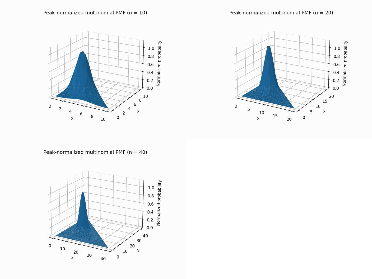

By taking $s$ to be large, we ensure there is a choice of a single tensor in the sum that captures the “bulk” of the complexity, allowing us to apply the simple case without “losing too much rank”.

Proof of the $\tau$-Theorem. Denote $\mathcal{T}=\bigoplus_{i=1}^{k}\langle n_{i},m_{i},p_{i} \rangle$. We are given $R(\mathcal{T}) \le r$. Consider the $s$-th power $\mathcal{T}^{\otimes s}$. By the sub-multiplicativity of rank, $R(\mathcal{T}^{\otimes s})\le r^{s}$.

Using the expansion derived above, for any fixed choice of exponents $\vec{a}=(a_{1},\dots,a_{k})$ summing to $s$, the specific term in the direct sum is a restriction of the whole. Thus: $$ R\left (\langle \mathcal{M}_{\vec{a}} \rangle \otimes \left\langle \prod_{i=1}^{k}n_{i}^{a_{i}}, \prod_{i=1}^{k}m_{i}^{a_{i}},\prod_{i=1}^{k}p_{i}^{a_{i}} \right\rangle\right) \le R(\mathcal{T}^{\otimes s}) \le r^{s} $$ This is exactly the setup for the Simple Case of the $\tau$-theorem (where the “multiplicity” is the multinomial coefficient). Applying the simple case result: $$ \mathcal{M}_{\vec{a}} \cdot \left(\prod_{i=1}^{k}(n_{i}m_{i}p_{i})^{a_{i}}\right)^{\omega/3} \le r^{s} $$ This inequality holds for every valid sequence $\vec{a}$. Summing over all possible choices of $\vec {a}$, and by the scalar multinomial theorem, we obtain: $$ \sum_{a_{1}+\dots+a_{k}=s} \binom{s}{a_{1},\dots,a_{k}} \cdot \prod_{i=1}^{k}\left((n_{i}m_{i}p_{i})^{\omega/3}\right)^{a_{i}} = \left(\sum_{i=1}^{k}(n_{i}m_{i}p_{i})^{\omega/3}\right)^{s} $$

The number of terms in the sum is equal to the number of solutions to $a_1 + \dots + a_k = s$, which is $\binom{k+s-1}{s-1}$. Thus, by averaging, there must exist at least one choice of $\vec{a}$ for which the term is at least the average value: $$ \text{Max Term} \ge \frac{\text{Sum}}{\text{Count}} \implies r^s \ge \text{Max Term} \ge \frac{\left(\sum_{i=1}^{k}(n_{i}m_{i}p_{i})^{\omega/3}\right)^{s}}{\binom{k+s-1}{s-1}} $$ Re-arranging and taking the $s$-th root, we see $$ \sum_{i=1}^{k}(n_{i}m_{i}p_{i})^{\omega/3} \le r \cdot \sqrt[s]{\binom{k+s-1}{s-1}} $$ Note that $\binom{k+s-1}{s-1}$ is a polynomial in $s$ of degree $k-1$. Specifically, it is roughly $s^{k-1}/(k-1)!$. Since $k$ is constant with respect to $s$, and it holds $\lim_{s\to \infty} \sqrt[s]{\text{Poly}_k (s)} = 1$ for any fixed polynomial of degree $k$, taking the limit of the inequality above $s \to \infty$ yields: $$ \sum_{i=1}^{k}(n_{i}m_{i}p_{i})^{\omega/3} \le r $$ $\blacksquare$

References

1. Bürgisser, P., Clausen, M., & Shokrollahi, M. A. (1997). Algebraic Complexity Theory .
2. Bläser, M. (2013). Fast Matrix Multiplication . 3 Schönhage, A. (1981). Partial and Total Matrix Multiplication .
3. Alman, J. Lecture Notes .